Tips and Tricks of Advanced Excel Pivot Table

Did you know what is PIVOT TABLE?

A Advance excel pivot table is a statistics as well as reporting tool that summarizes, analyse and reorganizes the data in a spreadsheet or database table to obtain a desired and meaningful report. The tool does not actually change the spreadsheet or database itself, it simply “pivots” or turns the data to view it from different perspectives.

Note: If you delete your raw data it does not reflect pivot table because it creates pivot cache in backend which save your reports and analysis.

Pivot tables are especially useful with large amounts of data and it is very time efficient tool to do large work in just a minute. A pivot table can perform include identifying sums, averages, ranges or outliers, percentages, charts, data analysis and many more in just drop and drag which is very easy and efficient for any user. The table then arranges this information in a simple, meaningful layout that draws attention to key values.

Pivot table is a generic term, but is sometimes confused This refers to a tool specific to Excel for creating pivot tables and pivot table is a part of Advance Excel. So, do you want to get best Advance excel online Training check here.
And learn some exciting and useful Tips and Tricks of Pivot Table listed below:

Tips & Tricks of Pivot Table

Table of Contents :
How to create Pivot Table
No blank row and column in data source.
Preserve Cell Formatting & disable auto-width in Pivot Table
Hide/Unhide subtotals and grand totals
Turn off/on (field list/ buttons/ field headers)
Insert slicer and Timeline
one slicer for all pivot table
creating many pivot table using filter pane option
Add Different values of same field
show values as Aggregation

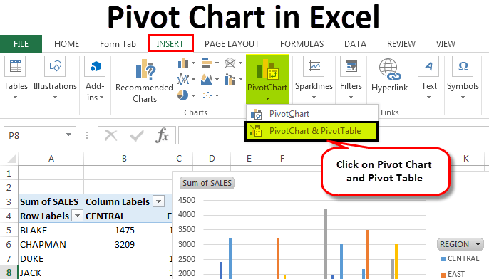
# How To Create Pivot Table

1. Click on insert tab.
2. Select pivot table option.
3. Select option table or range.
4. If we create pivot table on new worksheet then select new worksheet option otherwise select existing worksheet and give the location of data.
5. Press ok to create pivot table .

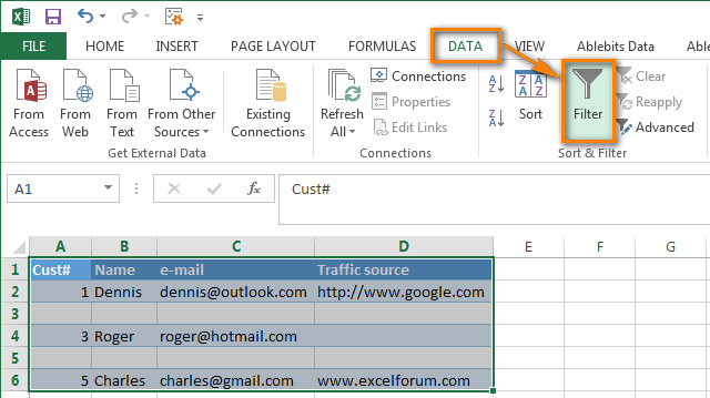
# No Blank Row and Column in Data Source.

One of the important things you need to keep in mind. check in the source data that there is any blank row or column.

If any row and column is blank then excel will not allow to create a perfect pivot table and Excel will only take data up to that row or column.

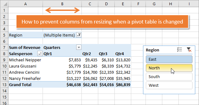
# Preserve Cell Formatting & Disable Auto-Width in Pivot Table

>Go to pivot table
>right click on pivot table
> go to pivot table option
>tick the options (preserve cell formatting on update)
>tick disable autofit column options
> then click ok to update
Note: The benefit of this option is whenever you update your pivot table you won’t lose the formatting you have. This option preserve your formatting as it is.

# Hide/Unhide subtotals and grand totals

When you add one or more column field in pivot table you will get subtotals and grand total automatic for the main field.

But if you don’t want subtotal and grand total you can hide them using steps below:

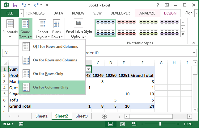
#Hide/Unhide subtotals for 2016 edition

>click on pivot table
>select design tab
>In the design tab
>go to Layout ➜ Subtotals ➜ Do not show subtotals.

#Hide/Unhide Grand Totals for 2016 Edition

>Click on the pivot table and go to the design tab
>In the design tab,
>go to Layout ➜ Grand Total ➜ Off for Rows and Columns.

#Turn off/on (field list/ buttons/ field headers)

Just like normal filters, expand/collapse and window pane of field list options in excel spreadsheets. In pivot table you can turn on/off filters, field list, buttons
Follow these steps:
Go to Analyze Tab
Choose field list/ button/ field headers and click
By clicking you can on/off these things.

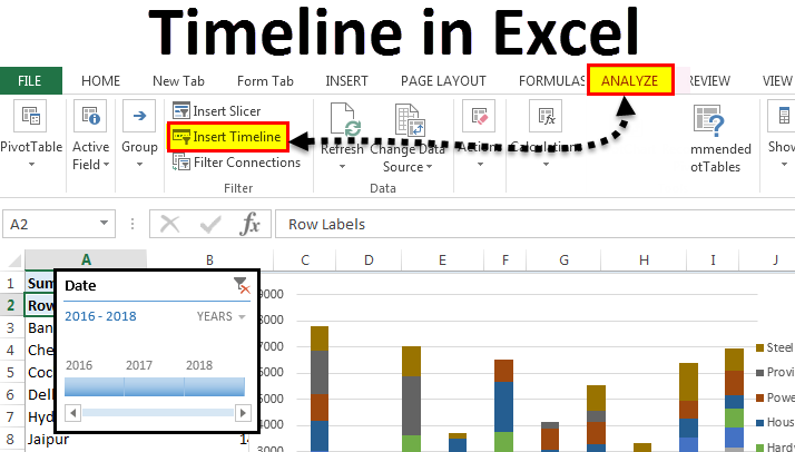
#Insert Slicer and Timeline

• Add Slicer : it is the best way to filter your data in Excel which is present in pivot table. By using slicer you can filter your data by any field whether the field is added in pivot table or not it can filter your data.
  Steps to add slicer:
  >go to Analyze Tab
  >In “Filter” group click on Insert slicer
  >click ok
• Add Timeline : A timeline is a special filter tool to filter the dates and become more powerful than normal filter. . Pivot table timelines allow you to quickly filter out your pivot table according to dates and time.
  Steps to add timeline:
  >go to Analyze Tab
  >In “filter” group click on insert timeline
  >click ok

# One Slicer for All Pivot Table

Whenever you have multiple pivot table related to each other. it’s hard to control all but adding slicer with relationship we can control/filter all pivot table with one slicer.
Steps for creating connection :
>create two or more pivot table with same data.
>go to analyze tab
>in “filter” group choose insert slicer
>after that “right click” on slicer
>choose option report connection
>then choose pivot tables you want to connect with slicer
>click ok

#Creating Many Pivot Table Using Filter Pane Option

If you want to create many pivot tables by filter pane option for ex : suppose you want to create pivot tables according to different product category and you have already created month wise sales pivot table and now you want to create three diffrent pivot table (month-wise sales) filtered by category so, with the “show report filter pages” option, we can create multiple worksheet with a pivot table for each product category.
follow steps for creating:
>Adding fields in pivot table “order date” in rows, “sales” in values, and “category” in filter pane
> after adding go to analyze tab
> choose “pivot table” then choose “options”
> In option choose “show report filter page”
>then click ok for creating multiple pivot table by category

#Add Different Values of Same Field

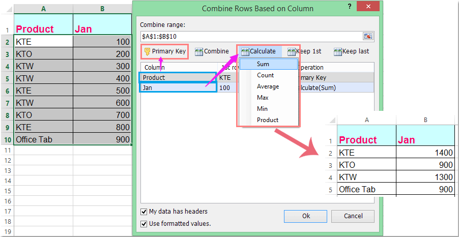
Whenever you want to add (sum and count) simultaneously in pivot table then, you have to choose value field setting options. Here, you can choose (max, min, count, sum, averages) etc…
Steps:
>create pivot table.
>then drag/add one value field in value pane.
>by default it shows (SUM) of any numeric field in values pane.
>by selecting down arrow option in value pane.
>go to value field setting.
>choose the value options you want like:(COUNT).
>click ok to add a count field in pivot table
>go to pivot table again add same numeric field in value pane.
>now, you can see both count of sales and sum of sales bot in same pivot.

#Show Values as Aggregation

Most of the time one or more aggregation is needed like (sum of sales, % of total sales) in you pivot table so here we can use “show value as” options. By this option we can show one or more calculations of same field/column.
Steps:
>create pivot table.
>then drag/add one value field in value pane.
>by default it shows (SUM) of any numeric field in values pane.
>by selecting down arrow option in value pane.
>go to value field setting.
>click on show value as option
>select any calculation (% of total)
>click ok then go to pivot table and again drag same field(sales).
>now you can see both sum of sales and % of total sales is added in pivot table

Enquire Now